You need a “good” optic that provides a “good” beam angle and a “good” color mixing. You know how to specify what a “good” beam angle should be, thanks to the full width half-maximum (FWHM). But how do you specify what a “good” color mixing should be?
We want to save you the hassle crawling on scientific literature for hours without finding anything relevant. This is why we developed a new and innovative technique to quantify the small colorimetric changes within a light distribution that makes a light beam appear “not good” from a color consistency standpoint.
This technique is called “Color Consistency Index“. It is an extension of the well-known MacAdam ellipses, applied to a continuous 2D light distribution. It can discriminate and sort out light distributions based on their colorimetric characteristics.
CIE 1931 diagram, chromaticity coordinates and MacAdam ellipses
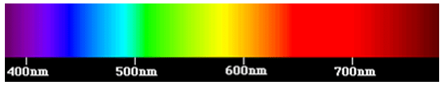
The Color Consistency Index is based upon physics and colorimetry, so let’s review the basics of colorimetry first. The visible light is only a small fraction of the electromagnetic radiations, the human eye can only see wavelengths from 380nm (violet) to 780nm (deep red)
Figure 1 - The visible spectrum I goes from 380nm to 780nm
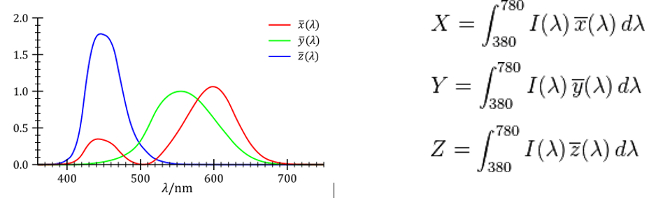
The visible light is converted by the human eye retina sensors into three stimuli X, Y, Z. The retina sensors are called “cones” and there are three kind of cones : one cone for the red (X), one cone for the green (Y) and one cone for the blue (Z).
The visible light is converted by the human eye retina sensors into three stimuli X, Y, Z. The retina sensors are called “cones” and there are three kind of cones : one cone for the red (X), one cone for the green (Y) and one cone for the blue (Z).
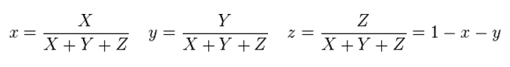
These three stimuli X, Y, Z generate a three-dimensional color space, which is too complex to handle. Therefore the three stimuli shall be normalized in order to separate the absolute luminance from the relevant color information. This normalization step is performed by the following operation.
Figure 3 - Normalized x, y stimuli
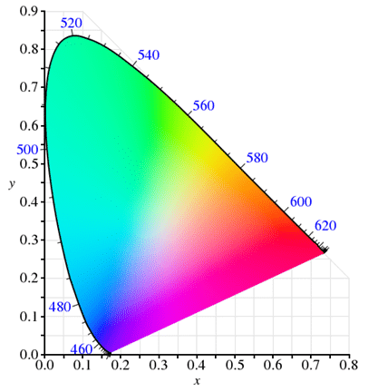
The normalized z stimuli may be obtained only from x and y, therefore the three-dimensional color space is now reduced to a two-dimensional space. This is how the (x, y) color space (also known as CIE1931 color space) is obtained. When plotted on a two-dimensional picture, we get the famous “horseshoe” diagram, as shown below.
Figure 4 - CIE 1931 (x,y) two-dimensional diagram
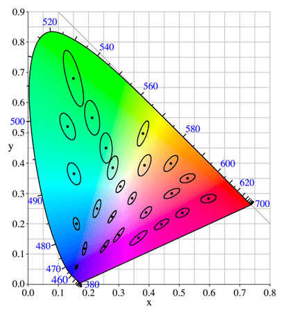
Now let’s consider two adjacent color shades inside this diagram. How can the eye discriminate two adjacent color shades ? David MacAdam answered this question in 1949. He conducted experimentations on a representative population. Then based on the results, he defined 25 ellipses with different sizes and orientations, in which two color shades may not be discriminated by an average human eye.
This is how the MacAdam ellipses are defined : MacAdam ellipses are areas of the CIE1931 diagram, in which two color shades may not be differentiated.
Figure 5 - MacAdam ellipses in the CIE 1931 diagram. The ellipses are 10 times their real size
These ellipses greatly help to understand how sensitive the human eye is. However the ellipses have non-constant size and orientation, which makes them difficult to use in practical experience. Ideally, constant-sized circles would be needed for metrology equipments.
For this reason, another color space was defined in which the human eye sensitivity is more even. The idea is to apply a reversible non-linear transformation in order to “distort” the color space. This is how the CIE1976 color space was defined, it is another color space derived from CIE1931 in which the human eye has a more constant sensitivity. The transformations from one color space to the other are given by the following formulas.
Figure 6 - CIE1931 to CIE1976 direct transformation
Figure 7 - CIE1976 to CIE1931 reverse transformation
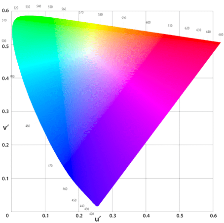
Two new stimuli u’ and v’ are obtained through the direct transformation. When plotted, we obtain the CIE1976 color space, as shown below.
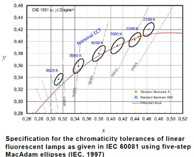
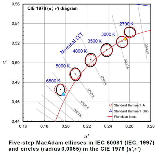
In the CIE1976 diagram, MacAdam ellipses are more uniform, with comparable size and orientation, although they are not perfectly identical. In particular, if we have a closer look to the white shades, also known as the black body locus or Planckian locus, then the MacAdam ellipses can be assimilated to constant circles.
Figure 9 – MacAdam ellipses next to the white shades in CIE1931 (left) and CIE1976 (right)
Figure 9 shows that in the CIE1976 diagram, next to the black body locus (where all the white shades are located) the MacAdam ellipses are equivalent to circles with a D=0.0022 constant diameter. Therefore a convenient way to check if two different white light sources may be discriminated is to compute the distance D between these two white light sources in the CIE1976 diagram. If the distance D is lower than D=0.0022, then the two whites light sources may not be discriminated.
Figure 10 - Discriminating two white shades in the CIE1976 diagram
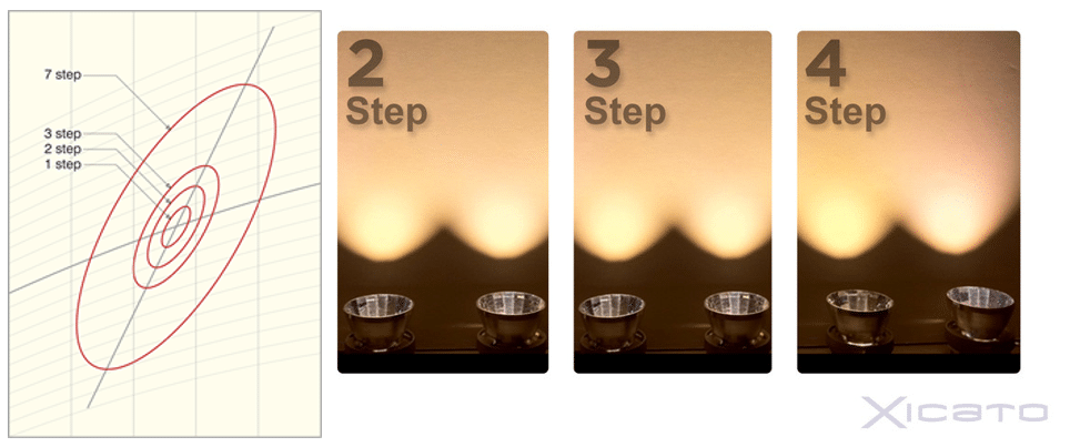
This is how the n-step MacAdam ellipses are defined :
Consider two different white light sources (1) and (2)
Measure their chromaticity coordinates (x1 y1) and (x2 y2) in the CIE 1931 diagram
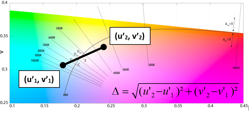
Convert (x1 y1) and (x2 y2) into (u’1 v’1) and (u’2 v’2) in the CIE 1976 diagram
Compute the distance between (u’1 v’1) and (u’2 v’2)
Compute n = / 0.0022
The result is the number of MacAdam ellipse steps. The higher the N-steps, the greater the visual difference between two white light sources
Figure 11 - n-steps MacAdam ellipses
The Color Consistency Index approach
The n-step MacAdam ellipse is a commonly used technique to discriminate individual white light sources. All LED manufacturers use it to define their color bins for white LEDs. However our topic is a little bit different. The topic is not to discriminate two different white light sources, the topic is to measure color variations inside a single light distribution.
So how shall we do ???
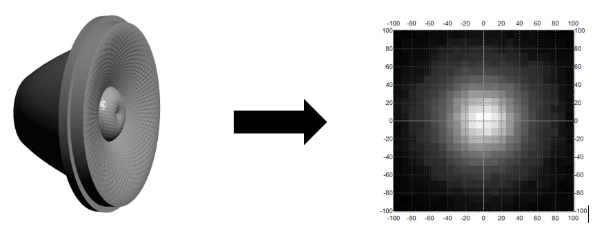
The idea is to extend the n-step ellipse concept, from two discrete points to a continuous distribution. Instead of considering the distance between two discrete points, the standard deviation of a continuous distribution shall be considered. Let’s consider a white luminaire projecting a whitish light distribution on a screen. The idea is to take a « picture » of the illuminance distribution and treat all pixels from this picture as elementary white light sources. Then the standard deviation from all pixels is computed and translated into MacAdam ellipses. This is how the Color Consistency Index is built, it is an extension of the MacAdam ellipses.
Figure 12 - Processing a single light distribution as a collection of pixels
The Color Consistency Index (CCI) shall be computed as follows.
1. Display a white color, from 2700°K to 6500°K, preferably 6000°K
In other words, consider a white resulting light, not some fancy colors.
The technique assumes that MacAdam ellipses are constant radius circles in the CIE1976 diagram. However, in the CIE1976 diagram, MacAdam ellipses may be assimilated to circles with a constant radius only for white shades, next to the black body locus. This can be seen on figure 9. For any other colors, especially for saturated colors, MacAdam ellipses still vary in size and orientation.
The ideal situation is to consider “perfect” white, which corresponds to a correlated color temperature of 6000°K (x=1/3 and y=1/3 in the CIE1931 diagram). However any white shade from 6500°K to 2700°K is still valid.
2. Map the chromaticity coordinates with a calibrated video-colorimeter
In other words, project the light distribution on a white screen and “take a picture” of it with a calibrated metrology equipment.
As for any physical measurement, a proper laboratory equipment is needed. A calibrated luminance meter / video-colorimeter shall be used for the measurement. The requirements are as follows :
Calibrated for luminance/illuminance, with linear sensitivity
Calibrated for chromaticity, in CIE1931 (x, y) or CIE1976 (u’, v’) diagram
Regular digital cameras use hidden signal transformations in order to make pictures look better. These signal transformations, on which the user has no control, are typically : Raw non-calibrated signal XYZ => Linear matrix transform RGB => Automatic white balance => Non-linear gamma correction sRGB. One can understand that computing (x, y) chromaticity coordinates with such altered data may be hazardous. Therefore a webcam or a smartphone may not be used !!!
3. Skip all pixels which are less than 10% of the maximum illuminance
In other words, the pixels with lower energy are not significant and shall not be considered.
Computing the (x, y) color coordinates out of a 12-bit depth digital image may be tricky. The (x, y) color coordinates shall be calculated out of the original X, Y, Z stimuli with the following formulas : x=X/(X+Y+Z) and y= x=Y/(X+Y+Z). If the X, Y, Z stimuli are too low, which occurs in dark areas with low signal, then the quantification process from the 12-bit digitization will induce a significant noise in the calculation. This is like computing A/B limit with A and B getting simultaneously to zero.
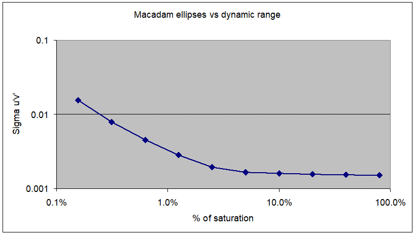
The graph below comes from a measurement made with a 12-bit calibrated video-colorimeter. A white light distribution with a good-but-not-perfect uniformity was measured for several exposure times. Then the standard deviation of the (u’, v’) mean color point was computed for each exposure time. 100% saturation means that the camera signal reaches 4096 value.
Figure 13 - Influence of the dynamic range on the color coordinates measurement precision.
Figure 13 shows that the measurement is stable beyond 5% and is altered below 5%. Therefore it is safe to consider only pixels that represent >10% of the maximum illuminance, and adjust the maximum illuminance to >50% of the camera saturation. Any pixel lower than 10% of the maximum illuminance shall be skipped.
This 10% threshold has another interpretation. In classical photometry, the intensity distribution is characterized with the Full Width Half Maximum angle (FWHM) and the Full Width Tenth percent of the Maximum angle (FWTM). It is commonly agreed that the FWTM value represents the main light distribution as the human eye perceives it. Skipping all pixels lower than 10% of the maximum illuminance means that only the main light distribution, as the human eye perceives it, is taken into account in the calculation.
4. Weight the pixels by the relative illuminance
In other words, more importance is granted to the brighter pixels.
All day life experience shows that color uniformity issues are more obvious for the human eye when the illuminance is higher. For this reason, when performing operations on the chromaticity coordinates, each step of the calculation shall be weighted by the illuminance.
5. For all significant pixels, compute the average colorimetric point in XY space (x0, y0)
Now it is time to compute the result. In order to compute the standard deviation, we need first to compute the mean value.
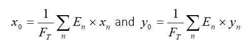
We shall first compute the Total Flux where En is the illuminance for the nth pixel.
Then we shall compute the Mean Color Point (x0, y0). This shall be done in the CIE1931 xy diagram only, because CIE1931 xy is a linear color space, while CIE1976 u’v’ is a non-linear color space. However doing the calculation in CIE1931 xy or CIE1976 u’v’ makes little or no difference in practical experience.
Then the Mean Color Point (x0, y0), weighted by the illuminance, shall be computed as follows.
Figure 14 - Computing the mean value in CIE1931 xy color space
When the illuminance is constant (En=constant), one can remark that the formula is a mean value calculation.
Remember that any pixel lower than 10% of the maximum illuminance shall be skipped.
6. For all significant pixels, compute the standard deviation in U'V' space: u’v’
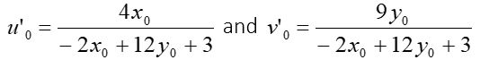
The Mean Color Point (x0, y0) shall be translated into CIE1976 (u’0, v’0) color coordinates, with the following formulas :
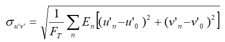
Then the standard deviation su’v’, weighted by the illuminance, shall be computed as follows.
Figure 15 - Computing the standard deviation in CIE1976 u'v' color space
When the illuminance is constant (En=constant), one can remark that the formula is a standard deviation calculation.
Remember that any pixel lower than 10% of the maximum illuminance shall be skipped.
7. Interpreting the results
The Color Consistency Index (CCI) is the standard deviation su’v’, computed as per figure 15. It is a number that typically varies from 0.001 up to 0.050.
The Color Consistency Index (CCI) is an extension of the n-step MacAdam ellipse concept, applied to a continuous white light distribution. In practical experience, it behaves like n-step MacAdam ellipses, the equivalent n-step MacAdam ellipse being n = su’v’ /0.0011.
N-step MacAdam ellipses
Color Consistency Index (CCI)
Colorimetry defects are…
1
CCI < 0.0016
Not visible to the eye
from 2 to 4
0.0017< CCI <0.0049
Hardly visible to the eye
5 and more
CCI > 0.0050
Clearly visible to the eye
Frequently Asked Questions
Most frequent questions and answers
Why did you choose this approach and why didn't you develop a method which takes more physical parameters into account ?
The idea is to use a known physical concept which is familiar to people in the lighting industry, and extend it to the problematic of color uniformity and color mixing. We are afraid that only few people would understand and assimilate a new technique based on complex signal processing and obscure calculations.
Could you share a few measurements made with this technique ?
You may visit our website https://www.optic-gaggione.com/products/ and browse our standard optic portfolio. Most of our color mixing optics are characterized with the Color Consistency Index.
May I use the Color Consistency Index to characterize the color-over-angle of my white static luminaire ?
Of course ! The technique was initially developed for RGBW color mixing applications, but it also works with tunable white luminaires as well as white static luminaires. If you can define a color correlated temperature for your luminaire, then you may characterize it with the Color Consistency Index.
So the Color Consistency Index characterizes the quality of an optical component, right ?
Not exactly, the Color Consistency Index measures the association of a light source (LED) and an optical component (collimator). In order to get a good color mixing, you need a good LED and a good collimator. The quality of the alignment and assembling also impacts the color mixing quality.